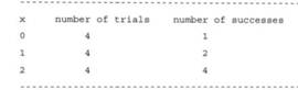
Refer to the following artificial data:
Denote by M0 the logistic null model and by M1 the model that also has x as a predictor. Denote the maximized log-likelihood values by L0 for M0, L1 for M1, and Ls for the saturated model. Create a data file in two ways, entering the data as (i) ungrouped data: 12 individual binary observations, (ii) grouped data: 3 summary binomial observations each with sample size = 4.
a. Fit M0 and M1 for each data file. Report L0 and L1 (or −2L0 and −2L1) in each case. Do they depend on the form of data entry?
b. Show that the deviances for M0 and M1 depend on the form of data entry. Why is this? (Hint: The saturated model has 12 parameters for data file (i) but 3 parameters for data file (ii).)
c. Show that the difference between the deviances does not depend on the form of data file. Thus, for testing the effect of x, it does not matter how you enter the data.

Ans:-
a) The parametric approach to statistical modeling assumes a family of probability distributions, such as the binomial, for the response variable. For a particular family, we can substitute the observed data into the formula for the probability function and then view how that probability depends on the unknown parameter value. For example, in n = 10 trials, suppose a binomial count equals y = 0. From the binomial formula (1.1) with parameter π, the probability of this outcome equals : P (0) = [10!/(0!)(10!)]π0(1 − π )10 = (1 − π )10
This probability is defined for all the potential values of π between 0 and 1. The probability of the observed data, expressed as a function of the parameter, is called the likelihood function. With y = 0 successes in n = 10 trials, the binomial likelihood function is l(π ) = (1 − π )10. It is defined for π between 0 and 1. From the likelihood function, if π = 0.40 for instance, the probability that Y = 0 is l(0.40) = (1 − 0.40)10 = 0.006. Likewise, if π = 0.20 then l(0.20) = (1 − 0.20)10 = 0.107, and if π = 0.0 then l(0.0) = (1 − 0.0)10 = 1.0. Figure 1.1 plots this likelihood function. The maximum likelihood estimate of a parameter is the parameter value for which the probability of the observed data takes its greatest value. It is the parameter value at which the likelihood function takes its maximum. Figure 1.1 shows that the likelihood function l(π ) = (1 − π )10 has its maximum at π = 0.0. Thus, when n = 10 trials have y = 0 successes, the maximum likelihood estimate of π equals 0.0. This means that the result y = 0 in n = 10 trials is more likely to occur when π = 0.00 than when π equals any other value. In general, for the binomial outcome of y successes in n trials, the maximum likelihood estimate of π equals p = y/n. This is the sample proportion of successes for the n trials. If we observe y = 6 successes in n = 10 trials, then the maximum likelihood estimate of π equals p = 6/10 = 0.60.
b) For a relatively small change in a quantitative predictor, Section 4.1.1 used a straight line to approximate the change in the probability. This simpler interpretation applies also with multiple predictors. Consider a setting of predictors at which P (Y ˆ = 1) = ˆπ. Then, controlling for the other predictors, a 1-unit increase in xj corresponds approximately to a βˆ jπ (ˆ 1 − ˆπ ) change in πˆ . For example, for the horseshoe crab data with predictors x = width and an indicator c that is 0 for dark crabs and 1 otherwise, logit(π )ˆ = −12.98 + 1.300c + 0.478x. When πˆ = 0.50, the approximate effect on πˆ of a 1 cm increase in x is (0.478)(0.50)(0.50) = 0.12. This is considerable, since a 1 cm change in width is less than half its standard deviation (which is 2.1 cm). This straight-line approximation deteriorates as the change in the predictor values increases. More precise interpretations use the probability formula directly. One way to describe the effect of a predictor xj sets the other predictors at their sample means and finds πˆ at the smallest and largest xj values. The effect is summarized by reporting those πˆ values or their difference. However, such summaries are sensitive to outliers on xj . To obtain a more robust summary, it is more sensible to use the quartiles of the xj values. For the prediction equation logit(π )ˆ = −12.98 + 1.300c + 0.478x, the sample means are 26.3 cm for x = width and 0.873 for c = color. The lower and upper quartiles of x are LQ = 24.9 cm and UQ = 27.7 cm. At x = 24.9 and c = ¯c, πˆ = 0.51. At x = 27.7 and c = ¯c, πˆ = 0.80. The change in πˆ from 0.51 to 0.80 over the middle 50% of the range of width values reflects a strong width effect. Since c takes only values 0 and 1, one could instead report this effect separately for each value of c rather than just at its mean.
c)
## Call:
## glm(formula = admit ~ gre + gpa + rank, family = "binomial",
## data = mydata)
##
## Deviance Residuals:
## Min 1Q Median 3Q Max
## -1.627 -0.866 -0.639 1.149 2.079
##
## Coefficients:
## Estimate Std. Error z value Pr(>|z|)
## (Intercept) -3.98998 1.13995 -3.50 0.00047 ***
## gre 0.00226 0.00109 2.07 0.03847 *
## gpa 0.80404 0.33182 2.42 0.01539 *
## rank2 -0.67544 0.31649 -2.13 0.03283 *
## rank3 -1.34020 0.34531 -3.88 0.00010 ***
## rank4 -1.55146 0.41783 -3.71 0.00020 ***
## ---
## Signif. codes: 0 '***' 0.001 '**' 0.01 '*' 0.05 '.' 0.1 ' ' 1
##
## (Dispersion parameter for binomial family taken to be 1)
##
## Null deviance: 499.98 on 399 degrees of freedom
## Residual deviance: 458.52 on 394 degrees of freedom
## AIC: 470.5
##
## Number of Fisher Scoring iterations: 4
In the output above, the first thing we see is the call, this is R reminding us what the model we ran was, what options we specified, etc.
Next we see the deviance residuals, which are a measure of model fit. This part of output shows the distribution of the deviance residuals for individual cases used in the model. Below we discuss how to use summaries of the deviance statistic to assess model fit.
The next part of the output shows the coefficients, their standard errors, the z-statistic (sometimes called a Wald z-statistic), and the associated p-values. Both gre and gpa are statistically significant, as are the three terms for rank. The logistic regression coefficients give the change in the log odds of the outcome for a one unit increase in the predictor variable.


